import warnings
warnings.filterwarnings('ignore')
warnings.simplefilter('ignore')Space X Falcon 9 First Stage Landing Prediction
Assignment: Machine Learning Prediction
Estimated time needed: 60 minutes
Space X advertises Falcon 9 rocket launches on its website with a cost of 62 million dollars; other providers cost upward of 165 million dollars each, much of the savings is because Space X can reuse the first stage. Therefore if we can determine if the first stage will land, we can determine the cost of a launch. This information can be used if an alternate company wants to bid against space X for a rocket launch. In this lab, you will create a machine learning pipeline to predict if the first stage will land given the data from the preceding labs.

Several examples of an unsuccessful landing are shown here:

Most unsuccessful landings are planed. Space X; performs a controlled landing in the oceans.
Objectives
Perform exploratory Data Analysis and determine Training Labels
create a column for the class
Standardize the data
Split into training data and test data
Find best Hyperparameter for SVM, Classification Trees and Logistic Regression
Find the method performs best using test data
Import Libraries and Define Auxiliary Functions
We will import the following libraries for the lab
# Pandas is a software library written for the Python programming language for data manipulation and analysis.
import pandas as pd
# NumPy is a library for the Python programming language, adding support for large, multi-dimensional arrays and matrices, along with a large collection of high-level mathematical functions to operate on these arrays
import numpy as np
# Matplotlib is a plotting library for python and pyplot gives us a MatLab like plotting framework. We will use this in our plotter function to plot data.
import matplotlib.pyplot as plt
#Seaborn is a Python data visualization library based on matplotlib. It provides a high-level interface for drawing attractive and informative statistical graphics
import seaborn as sns
# Preprocessing allows us to standarsize our data
from sklearn import preprocessing
# Allows us to split our data into training and testing data
from sklearn.model_selection import train_test_split
# Allows us to test parameters of classification algorithms and find the best one
from sklearn.model_selection import GridSearchCV
# Logistic Regression classification algorithm
from sklearn.linear_model import LogisticRegression
# Support Vector Machine classification algorithm
from sklearn.svm import SVC
# Decision Tree classification algorithm
from sklearn.tree import DecisionTreeClassifier
# K Nearest Neighbors classification algorithm
from sklearn.neighbors import KNeighborsClassifier
/home/jupyterlab/conda/envs/python/lib/python3.7/site-packages/sklearn/utils/validation.py:37: DeprecationWarning: distutils Version classes are deprecated. Use packaging.version instead.
LARGE_SPARSE_SUPPORTED = LooseVersion(scipy_version) >= '0.14.0'
/home/jupyterlab/conda/envs/python/lib/python3.7/site-packages/sklearn/linear_model/least_angle.py:35: DeprecationWarning: `np.float` is a deprecated alias for the builtin `float`. To silence this warning, use `float` by itself. Doing this will not modify any behavior and is safe. If you specifically wanted the numpy scalar type, use `np.float64` here.
Deprecated in NumPy 1.20; for more details and guidance: https://numpy.org/devdocs/release/1.20.0-notes.html#deprecations
eps=np.finfo(np.float).eps,
/home/jupyterlab/conda/envs/python/lib/python3.7/site-packages/sklearn/linear_model/least_angle.py:597: DeprecationWarning: `np.float` is a deprecated alias for the builtin `float`. To silence this warning, use `float` by itself. Doing this will not modify any behavior and is safe. If you specifically wanted the numpy scalar type, use `np.float64` here.
Deprecated in NumPy 1.20; for more details and guidance: https://numpy.org/devdocs/release/1.20.0-notes.html#deprecations
eps=np.finfo(np.float).eps, copy_X=True, fit_path=True,
/home/jupyterlab/conda/envs/python/lib/python3.7/site-packages/sklearn/linear_model/least_angle.py:836: DeprecationWarning: `np.float` is a deprecated alias for the builtin `float`. To silence this warning, use `float` by itself. Doing this will not modify any behavior and is safe. If you specifically wanted the numpy scalar type, use `np.float64` here.
Deprecated in NumPy 1.20; for more details and guidance: https://numpy.org/devdocs/release/1.20.0-notes.html#deprecations
eps=np.finfo(np.float).eps, copy_X=True, fit_path=True,
/home/jupyterlab/conda/envs/python/lib/python3.7/site-packages/sklearn/linear_model/least_angle.py:862: DeprecationWarning: `np.float` is a deprecated alias for the builtin `float`. To silence this warning, use `float` by itself. Doing this will not modify any behavior and is safe. If you specifically wanted the numpy scalar type, use `np.float64` here.
Deprecated in NumPy 1.20; for more details and guidance: https://numpy.org/devdocs/release/1.20.0-notes.html#deprecations
eps=np.finfo(np.float).eps, positive=False):
/home/jupyterlab/conda/envs/python/lib/python3.7/site-packages/sklearn/linear_model/least_angle.py:1097: DeprecationWarning: `np.float` is a deprecated alias for the builtin `float`. To silence this warning, use `float` by itself. Doing this will not modify any behavior and is safe. If you specifically wanted the numpy scalar type, use `np.float64` here.
Deprecated in NumPy 1.20; for more details and guidance: https://numpy.org/devdocs/release/1.20.0-notes.html#deprecations
max_n_alphas=1000, n_jobs=None, eps=np.finfo(np.float).eps,
/home/jupyterlab/conda/envs/python/lib/python3.7/site-packages/sklearn/linear_model/least_angle.py:1344: DeprecationWarning: `np.float` is a deprecated alias for the builtin `float`. To silence this warning, use `float` by itself. Doing this will not modify any behavior and is safe. If you specifically wanted the numpy scalar type, use `np.float64` here.
Deprecated in NumPy 1.20; for more details and guidance: https://numpy.org/devdocs/release/1.20.0-notes.html#deprecations
max_n_alphas=1000, n_jobs=None, eps=np.finfo(np.float).eps,
/home/jupyterlab/conda/envs/python/lib/python3.7/site-packages/sklearn/linear_model/least_angle.py:1480: DeprecationWarning: `np.float` is a deprecated alias for the builtin `float`. To silence this warning, use `float` by itself. Doing this will not modify any behavior and is safe. If you specifically wanted the numpy scalar type, use `np.float64` here.
Deprecated in NumPy 1.20; for more details and guidance: https://numpy.org/devdocs/release/1.20.0-notes.html#deprecations
eps=np.finfo(np.float).eps, copy_X=True, positive=False):
/home/jupyterlab/conda/envs/python/lib/python3.7/site-packages/sklearn/linear_model/randomized_l1.py:152: DeprecationWarning: `np.float` is a deprecated alias for the builtin `float`. To silence this warning, use `float` by itself. Doing this will not modify any behavior and is safe. If you specifically wanted the numpy scalar type, use `np.float64` here.
Deprecated in NumPy 1.20; for more details and guidance: https://numpy.org/devdocs/release/1.20.0-notes.html#deprecations
precompute=False, eps=np.finfo(np.float).eps,
/home/jupyterlab/conda/envs/python/lib/python3.7/site-packages/sklearn/linear_model/randomized_l1.py:320: DeprecationWarning: `np.float` is a deprecated alias for the builtin `float`. To silence this warning, use `float` by itself. Doing this will not modify any behavior and is safe. If you specifically wanted the numpy scalar type, use `np.float64` here.
Deprecated in NumPy 1.20; for more details and guidance: https://numpy.org/devdocs/release/1.20.0-notes.html#deprecations
eps=np.finfo(np.float).eps, random_state=None,
/home/jupyterlab/conda/envs/python/lib/python3.7/site-packages/sklearn/linear_model/randomized_l1.py:580: DeprecationWarning: `np.float` is a deprecated alias for the builtin `float`. To silence this warning, use `float` by itself. Doing this will not modify any behavior and is safe. If you specifically wanted the numpy scalar type, use `np.float64` here.
Deprecated in NumPy 1.20; for more details and guidance: https://numpy.org/devdocs/release/1.20.0-notes.html#deprecations
eps=4 * np.finfo(np.float).eps, n_jobs=None,This function is to plot the confusion matrix.
def plot_confusion_matrix(y,y_predict):
    "this function plots the confusion matrix"
    from sklearn.metrics import confusion_matrix

    cm = confusion_matrix(y, y_predict)
    ax= plt.subplot()
    sns.heatmap(cm, annot=True, ax = ax); #annot=True to annotate cells
    ax.set_xlabel('Predicted labels')
    ax.set_ylabel('True labels')
    ax.set_title('Confusion Matrix');
    ax.xaxis.set_ticklabels(['did not land', 'land']); ax.yaxis.set_ticklabels(['did not land', 'landed'])
Load the dataframe
Load the data
data = pd.read_csv("https://cf-courses-data.s3.us.cloud-object-storage.appdomain.cloud/IBM-DS0321EN-SkillsNetwork/datasets/dataset_part_2.csv")

# If you were unable to complete the previous lab correctly you can uncomment and load this csv

# data = pd.read_csv('https://cf-courses-data.s3.us.cloud-object-storage.appdomain.cloud/IBMDeveloperSkillsNetwork-DS0701EN-SkillsNetwork/api/dataset_part_2.csv')

data.head()| FlightNumber | Date | BoosterVersion | PayloadMass | Orbit | LaunchSite | Outcome | Flights | GridFins | Reused | Legs | LandingPad | Block | ReusedCount | Serial | Longitude | Latitude | Class | |
|---|---|---|---|---|---|---|---|---|---|---|---|---|---|---|---|---|---|---|
| 0 | 1 | 2010-06-04 | Falcon 9 | 6104.959412 | LEO | CCAFS SLC 40 | None None | 1 | False | False | False | NaN | 1.0 | 0 | B0003 | -80.577366 | 28.561857 | 0 |
| 1 | 2 | 2012-05-22 | Falcon 9 | 525.000000 | LEO | CCAFS SLC 40 | None None | 1 | False | False | False | NaN | 1.0 | 0 | B0005 | -80.577366 | 28.561857 | 0 |
| 2 | 3 | 2013-03-01 | Falcon 9 | 677.000000 | ISS | CCAFS SLC 40 | None None | 1 | False | False | False | NaN | 1.0 | 0 | B0007 | -80.577366 | 28.561857 | 0 |
| 3 | 4 | 2013-09-29 | Falcon 9 | 500.000000 | PO | VAFB SLC 4E | False Ocean | 1 | False | False | False | NaN | 1.0 | 0 | B1003 | -120.610829 | 34.632093 | 0 |
| 4 | 5 | 2013-12-03 | Falcon 9 | 3170.000000 | GTO | CCAFS SLC 40 | None None | 1 | False | False | False | NaN | 1.0 | 0 | B1004 | -80.577366 | 28.561857 | 0 |
X = pd.read_csv('https://cf-courses-data.s3.us.cloud-object-storage.appdomain.cloud/IBM-DS0321EN-SkillsNetwork/datasets/dataset_part_3.csv')

# If you were unable to complete the previous lab correctly you can uncomment and load this csv

# X = pd.read_csv('https://cf-courses-data.s3.us.cloud-object-storage.appdomain.cloud/IBMDeveloperSkillsNetwork-DS0701EN-SkillsNetwork/api/dataset_part_3.csv')

X.head(100)| FlightNumber | PayloadMass | Flights | Block | ReusedCount | Orbit_ES-L1 | Orbit_GEO | Orbit_GTO | Orbit_HEO | Orbit_ISS | ... | Serial_B1058 | Serial_B1059 | Serial_B1060 | Serial_B1062 | GridFins_False | GridFins_True | Reused_False | Reused_True | Legs_False | Legs_True | |
|---|---|---|---|---|---|---|---|---|---|---|---|---|---|---|---|---|---|---|---|---|---|
| 0 | 1.0 | 6104.959412 | 1.0 | 1.0 | 0.0 | 0.0 | 0.0 | 0.0 | 0.0 | 0.0 | ... | 0.0 | 0.0 | 0.0 | 0.0 | 1.0 | 0.0 | 1.0 | 0.0 | 1.0 | 0.0 |
| 1 | 2.0 | 525.000000 | 1.0 | 1.0 | 0.0 | 0.0 | 0.0 | 0.0 | 0.0 | 0.0 | ... | 0.0 | 0.0 | 0.0 | 0.0 | 1.0 | 0.0 | 1.0 | 0.0 | 1.0 | 0.0 |
| 2 | 3.0 | 677.000000 | 1.0 | 1.0 | 0.0 | 0.0 | 0.0 | 0.0 | 0.0 | 1.0 | ... | 0.0 | 0.0 | 0.0 | 0.0 | 1.0 | 0.0 | 1.0 | 0.0 | 1.0 | 0.0 |
| 3 | 4.0 | 500.000000 | 1.0 | 1.0 | 0.0 | 0.0 | 0.0 | 0.0 | 0.0 | 0.0 | ... | 0.0 | 0.0 | 0.0 | 0.0 | 1.0 | 0.0 | 1.0 | 0.0 | 1.0 | 0.0 |
| 4 | 5.0 | 3170.000000 | 1.0 | 1.0 | 0.0 | 0.0 | 0.0 | 1.0 | 0.0 | 0.0 | ... | 0.0 | 0.0 | 0.0 | 0.0 | 1.0 | 0.0 | 1.0 | 0.0 | 1.0 | 0.0 |
| ... | ... | ... | ... | ... | ... | ... | ... | ... | ... | ... | ... | ... | ... | ... | ... | ... | ... | ... | ... | ... | ... |
| 85 | 86.0 | 15400.000000 | 2.0 | 5.0 | 2.0 | 0.0 | 0.0 | 0.0 | 0.0 | 0.0 | ... | 0.0 | 0.0 | 1.0 | 0.0 | 0.0 | 1.0 | 0.0 | 1.0 | 0.0 | 1.0 |
| 86 | 87.0 | 15400.000000 | 3.0 | 5.0 | 2.0 | 0.0 | 0.0 | 0.0 | 0.0 | 0.0 | ... | 1.0 | 0.0 | 0.0 | 0.0 | 0.0 | 1.0 | 0.0 | 1.0 | 0.0 | 1.0 |
| 87 | 88.0 | 15400.000000 | 6.0 | 5.0 | 5.0 | 0.0 | 0.0 | 0.0 | 0.0 | 0.0 | ... | 0.0 | 0.0 | 0.0 | 0.0 | 0.0 | 1.0 | 0.0 | 1.0 | 0.0 | 1.0 |
| 88 | 89.0 | 15400.000000 | 3.0 | 5.0 | 2.0 | 0.0 | 0.0 | 0.0 | 0.0 | 0.0 | ... | 0.0 | 0.0 | 1.0 | 0.0 | 0.0 | 1.0 | 0.0 | 1.0 | 0.0 | 1.0 |
| 89 | 90.0 | 3681.000000 | 1.0 | 5.0 | 0.0 | 0.0 | 0.0 | 0.0 | 0.0 | 0.0 | ... | 0.0 | 0.0 | 0.0 | 1.0 | 0.0 | 1.0 | 1.0 | 0.0 | 0.0 | 1.0 |
90 rows × 83 columns
TASK 1
Create a NumPy array from the column Class in data, by applying the method to_numpy() then assign it to the variable Y,make sure the output is a Pandas series (only one bracket df[‘name of column’]).
Y = data.Class.to_numpy()TASK 2
Standardize the data in X then reassign it to the variable X using the transform provided below.
# students get this
transform = preprocessing.StandardScaler()
X = transform.fit_transform(X)Xarray([[-1.71291154e+00, -1.94814463e-16, -6.53912840e-01, ...,
-8.35531692e-01, 1.93309133e+00, -1.93309133e+00],
[-1.67441914e+00, -1.19523159e+00, -6.53912840e-01, ...,
-8.35531692e-01, 1.93309133e+00, -1.93309133e+00],
[-1.63592675e+00, -1.16267307e+00, -6.53912840e-01, ...,
-8.35531692e-01, 1.93309133e+00, -1.93309133e+00],
...,
[ 1.63592675e+00, 1.99100483e+00, 3.49060516e+00, ...,
1.19684269e+00, -5.17306132e-01, 5.17306132e-01],
[ 1.67441914e+00, 1.99100483e+00, 1.00389436e+00, ...,
1.19684269e+00, -5.17306132e-01, 5.17306132e-01],
[ 1.71291154e+00, -5.19213966e-01, -6.53912840e-01, ...,
-8.35531692e-01, -5.17306132e-01, 5.17306132e-01]])We split the data into training and testing data using the function train_test_split. The training data is divided into validation data, a second set used for training data; then the models are trained and hyperparameters are selected using the function GridSearchCV.
TASK 3
Use the function train_test_split to split the data X and Y into training and test data. Set the parameter test_size to 0.2 and random_state to 2. The training data and test data should be assigned to the following labels.
X_train, X_test, Y_train, Y_test
X_train, X_test, Y_train, Y_test = train_test_split(X, Y, test_size=0.2, random_state=2)we can see we only have 18 test samples.
Y_test.shape(18,)TASK 4
Create a logistic regression object then create a GridSearchCV object logreg_cv with cv = 10. Fit the object to find the best parameters from the dictionary parameters.
parameters ={'C':[0.01,0.1,1],
             'penalty':['l2'],
             'solver':['lbfgs']}
import warnings
warnings.filterwarnings('ignore')
warnings.simplefilter('ignore')parameters ={"C":[0.01,0.1,1],'penalty':['l2'], 'solver':['lbfgs']}# l1 lasso l2 ridge
lr=LogisticRegression()
logreg_cv = GridSearchCV(estimator=lr, param_grid=parameters, cv=10)
logreg_model_result = logreg_cv.fit(X_train, Y_train)We output the GridSearchCV object for logistic regression. We display the best parameters using the data attribute best_params_ and the accuracy on the validation data using the data attribute best_score_.
print("tuned hyperparameters :(best parameters) ",logreg_cv.best_params_)
print("accuracy :",logreg_cv.best_score_)
tuned hyperparameters :(best parameters) {'C': 0.01, 'penalty': 'l2', 'solver': 'lbfgs'}
accuracy : 0.8472222222222222TASK 5
Calculate the accuracy on the test data using the method score:
print("Accuracy of logistic regression classifier: ", logreg_cv.score(X_test, Y_test))Accuracy of logistic regression classifier: 0.8333333333333334Lets look at the confusion matrix:
yhat=logreg_cv.predict(X_test)
plot_confusion_matrix(Y_test,yhat)
Examining the confusion matrix, we see that logistic regression can distinguish between the different classes. We see that the major problem is false positives.
TASK 6
Create a support vector machine object then create a GridSearchCV object svm_cv with cv - 10. Fit the object to find the best parameters from the dictionary parameters.
parameters = {'kernel':('linear', 'rbf','poly','rbf', 'sigmoid'),
              'C': np.logspace(-3, 3, 5),
              'gamma':np.logspace(-3, 3, 5)}
svm = SVC()
svm_cv = GridSearchCV(estimator=svm, param_grid=parameters, cv=10)
svm_model_result = svm_cv.fit(X_train, Y_train)print("tuned hyperparameters :(best parameters) ",svm_cv.best_params_)
print("accuracy :",svm_cv.best_score_)tuned hyperparameters :(best parameters) {'C': 1.0, 'gamma': 0.03162277660168379, 'kernel': 'sigmoid'}
accuracy : 0.8472222222222222TASK 7
Calculate the accuracy on the test data using the method score:
print("Accuracy of support vector machine: ", svm_cv.score(X_test, Y_test))Accuracy of support vector machine: 0.8333333333333334We can plot the confusion matrix
yhat=svm_cv.predict(X_test)
plot_confusion_matrix(Y_test,yhat)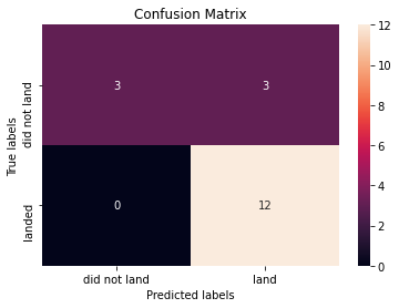
TASK 8
Create a decision tree classifier object then create a GridSearchCV object tree_cv with cv = 10. Fit the object to find the best parameters from the dictionary parameters.
parameters = {'criterion': ['gini', 'entropy'],
     'splitter': ['best', 'random'],
     'max_depth': [2*n for n in range(1,10)],
     'max_features': ['auto', 'sqrt'],
     'min_samples_leaf': [1, 2, 4],
     'min_samples_split': [2, 5, 10]}

tree = DecisionTreeClassifier()
tree_cv = GridSearchCV(estimator=tree, param_grid=parameters, cv=10)
tree_cv_model_result = tree_cv.fit(X_train, Y_train)print("tuned hpyerparameters :(best parameters) ",tree_cv.best_params_)
print("accuracy :",tree_cv.best_score_)tuned hpyerparameters :(best parameters) {'criterion': 'gini', 'max_depth': 2, 'max_features': 'sqrt', 'min_samples_leaf': 4, 'min_samples_split': 10, 'splitter': 'random'}
accuracy : 0.875TASK 9
Calculate the accuracy of tree_cv on the test data using the method score:
print("Accuracy of decision tree classifier: ", tree_cv.score(X_test, Y_test))Accuracy of decision tree classifier: 0.8333333333333334We can plot the confusion matrix
yhat = tree_cv.predict(X_test)
plot_confusion_matrix(Y_test,yhat)
TASK 10
Create a k nearest neighbors object then create a GridSearchCV object knn_cv with cv = 10. Fit the object to find the best parameters from the dictionary parameters.
parameters = {'n_neighbors': [1, 2, 3, 4, 5, 6, 7, 8, 9, 10],
              'algorithm': ['auto', 'ball_tree', 'kd_tree', 'brute'],
              'p': [1,2]}

KNN = KNeighborsClassifier()
knn_cv = GridSearchCV(estimator=KNN, param_grid=parameters, cv=10)
knn_cv_model_result = knn_cv.fit(X_train, Y_train)print("tuned hpyerparameters :(best parameters) ",knn_cv.best_params_)
print("accuracy :",knn_cv.best_score_)tuned hpyerparameters :(best parameters) {'algorithm': 'auto', 'n_neighbors': 9, 'p': 1}
accuracy : 0.8472222222222222TASK 11
Calculate the accuracy of knn_cv on the test data using the method score:
print("Accuracy of k nearest neighbors: ", knn_cv.score(X_test, Y_test))Accuracy of k nearest neighbors: 0.8333333333333334We can plot the confusion matrix
yhat = knn_cv.predict(X_test)
plot_confusion_matrix(Y_test,yhat)
TASK 12
Find the method performs best:
As all the algorithms are giving the same accuracy, they all perform practically the same.
Extra Task:
Bar Chart for all classification models
scores = {'logreg_cv':logreg_cv.score(X_test, Y_test), 'svm_cv':svm_cv.score(X_test, Y_test),
          'tree_cv':tree_cv.score(X_test, Y_test), 'knn_cv':knn_cv.score(X_test, Y_test)}

labels = list(scores.keys())
values = list(scores.values())

fig = plt.figure(figsize = (10, 5))
plt.bar(labels, values)
plt.xlabel("Model")
plt.ylabel("Accuracy")
plt.title("Classification Models")
plt.show()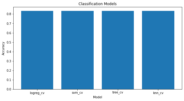
Change Log
| Date (YYYY-MM-DD) | Version | Changed By | Change Description |
|---|---|---|---|
| 2021-08-31 | 1.1 | Lakshmi Holla | Modified markdown |
| 2020-09-20 | 1.0 | Joseph | Modified Multiple Areas |
Copyright © 2020 IBM Corporation. All rights reserved.